4. Understand how a Neural Network works
4.1. Graphical Understanding


4.2. Simple Neural Network (1 hidden layer)
| import numpy as np # sigmoid function def nonlin(x,deriv=False): if(deriv==True): return x*(1-x) return 1/(1+np.exp(-x)) # input dataset X = np.array([ [0,0,1], [0,1,1], [1,0,1], [1,1,1] ]) # output dataset y = np.array([[0,0,1,1]]).T # seed random numbers to make calculation # deterministic (just a good practice) np.random.seed(1) # initialize weights randomly with mean 0 : Synapse 0 syn0 = 2*np.random.random((3,1)) - 1 # QUESTION for iter in range(10000): # forward propagation l0 = X l1 = nonlin(np.dot(l0,syn0)) # how much did we miss? l1_error = y - l1 # multiply how much we missed by the # slope of the sigmoid at the values in l1 l1_delta = l1_error * nonlin(l1,True) # update weights syn0 += np.dot(l0.T,l1_delta) print ("Output After Training:") print (l1) |
Imports numpy (linear algebra library), our only dependency. Activation of a neuron (sigmoid function, nonlinearity) Generates the derivative of a sigmoid (when deriv=True). The sigmoid output can be used to create its derivative. If it’s a variable “out”, then the derivative is out(1-out) X: Input dataset matrix, each row is a training example Training data (4 examples, 3 input nodes) y: Output dataset matrix, each row is a training example Label of every data (binary classification). Each row (4) is a training example, and each column (1) an output node. Numbers still randomly distributed but exactly the same way each time we train. Initialization of the weights (this neural network has 1 layer of weights: 3 input, 1 output). Every link value is stored in syn0. syn0: 1st layer of weights, connects l0 to l1 —> weight matrix (dimensions 3 by 1 since we have 3 inputs and 1 output: l0 is of size 3 and l1 of size 1) ! We don’t save layers, but “syn” matrices (they store the learning) Network training code begins here (iterated for optimization): l0: First Layer of the Network, specified by the input data l1 (second layer, hidden) is the prediction step. We let the network “try” to predict the output from the input, and we analyze results to perform better each iteration. Two steps: multiplication of l0 by syn0 & passing output through sigmoid function (defined before as nonlin) l1 had a “guess”, so we compare how it did by subtracting y (true answer) from l1 (guess), and we obtain a vector of positive and negative numbers nonlin(l1, True) generates the slopes of the lines of the dots represented by l1 Error weighted derivative: multiplies the points of l1 passed through the sigmoid function (nonlin…), by l1_error Updates weights by computing the update for each weight for each training example and summing them. Prints result |
| Output After Training: [[0.00966449] [0.00786506] [0.99358898] [0.99211957]] |
The code: Trains the neural network Passes every data Evaluates the error Updates the weights using back propagation |
4.3. Simple Neural Network (1 hidden layer, ReLU activation function)
| import numpy as np print("Enter the two values for input layers") print('a = ') a = int(input()) # 2 print('b = ') b = int(input()) weights = { 'node_0': np.array([2, 4]), 'node_1': np.array([[4, -5]]), 'output_node': np.array([2, 7]) } input_data = np.array([a, b]) def relu(input): # Rectified Linear Activation output = max(input, 0) return(output) node_0_input = (input_data * weights['node_0']).sum() node_0_output = relu(node_0_input) node_1_input = (input_data * weights['node_1']).sum() node_1_output = relu(node_1_input) hidden_layer_outputs = np.array([node_0_output, node_1_output]) model_output = (hidden_layer_outputs * weights['output_node']).sum() print(model_output) |
| Enter the two values for input layers a = 2 b = 3 32 |
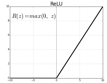 |
| Source: Sarkar, K. "ReLU: Not a differentiable function" |
4.4. Simple Neural Network (2 hidden layers)
| import numpy as np # sigmoid function def nonlin(x, deriv=False): if (deriv == True): return (x * (1 - x)) return 1 / (1 + np.exp(-x)) # input dataset X = np.array([ [1,1,1], [3,3,3], [2,2,2], [2,2,2] ]) # output dataset y = np.array([[1], [1], [0], [1]]) # seed random numbers to make calculation # deterministic (just a good practice) np.random.seed(1) # randomly initialize our weights #with mean 0 syn0 = 2*np.random.random((3,4)) - 1 syn1 = 2*np.random.random((4,1)) - 1 for j in range(60000): # Feed forward through layers 0, 1, and 2 l0 = X l1 = nonlin(np.dot(l0,syn0)) l2 = nonlin(np.dot(l1,syn1)) # how much did we miss the target value? l2_error = y - l2 if (j% 10000) == 0: print ('Error:' + str(np.mean(np.abs(l2_error)))) # in what direction is the target value? # were we really sure? if so, # don't change too much. l2_delta = l2_error*nonlin(l2,deriv=True) # how much did each l1 value contribute to the l2 error (according to the weights)? l1_error = l2_delta.dot(syn1.T) # in what direction is the target l1? # were we really sure? if so, #don't change too much. l1_delta = l1_error * nonlin(l1,deriv=True) syn1 += l1.T.dot(l2_delta) syn0 += l0.T.dot(l1_delta) print ('Output after training') print (l2) |
Imports numpy (linear algebra library), our only dependency. Activation of a neuron (sigmoid function, nonlinearity) Generates the derivative of a sigmoid (when derive=True). The sigmoid output can be used to create its derivative. If it’s a variable “out”, then the derivative is out(1-out) X: Input dataset matrix, each row is a training example Training data (4 examples, 3 input nodes) y: Output dataset matrix, each row is a training example Label of every data (binary classification). Each row (4) is a training example, and each column (1) an output node. Same as writing: y = np.array([[1,1,0,1]]).T Numbers still randomly distributed but exactly the same way each time we train. Initialization of the weights (this neural network has 2 layers of weights: 3 input neurons, 4 hidden, 1 output). The value of every link is stored in syn0 and syn1. syn0: 1st layer of weights, Synapse 0, connects l0 to l1 —> weight matrix (dimensions 3 by 4 since we have 3 inputs and 4 outputs: l0 is of size 3 and l1 of size 4) syn1: 2nd layer of weights, Synapse 1, connects l1 to l2. ! We don’t save layers, but “syn” matrices (they store the learning) Network training code begins here (iterated for optimization): l0: First Layer of the Network, specified by the input data l1 (2nd layer, hidden) and l2 (3rs layer, hidden) are the prediction step. We let the network “try” to predict the output from the input, and we analyze results to perform better each iteration. Two steps: multiplication of l0 by syn0 & passing output through sigmoid function. Compare how guess (l2) against real output value. The % is calculating the remainder between j and 1000, so that if it is zero, an error will be printed. This is done since we are iterating for j in range(6000) so we can get 6 recordings of the error computed (just for our information). Notice it must decrease, otherwise we are doing something wrong!!! Error weighted derivative nonlin(l2, True) generates the slopes of the lines of the dots represented by l2 Uses the “confidence weighted error” from l2 to establish an error for l1 (by sending the error across the weights from l2 to l1). We learn how much each node value in l1 “contributed” to the error in l2 (backpropagating step) Then syn0 update. |
| Error:0.49641003190272537 Error:0.008584525653247153 Error:0.005789459862507809 Error:0.004629176776769984 Error:0.003958765280273649 Error:0.003510122567861676 Output after training [[0.00260572] [0.99672209] [0.99701711] [0.00386759]] |
The code: Trains the neural network Passes every data Evaluates the error Updates the weights using back propagation |
4.5. Predicting Numbers from zero to three (simple NN with 2 hidden layers)
| import numpy as np zero = [ 0, 1, 1, 0, 1, 0, 0, 1, 1, 0, 0, 1, 1, 0, 0, 1, 0, 1, 1, 0 ] one = [ 0, 0, 1, 0, 0, 0, 1, 0, 0, 0, 1, 0, 0, 0, 1, 0, 0, 0, 1, 0 ] two = [ 0, 1, 1, 0, 1, 0, 0, 1, 0, 0, 1, 0, 0, 1, 0, 0, 1, 1, 1, 1 ] three = [ 1, 1, 1, 1, 0, 0, 0, 1, 0, 1, 1, 1, 0, 0, 0, 1, 1, 1, 1, 1] predict = [ 0, 1, 1, 0, 1, 0, 0, 1, 0, 0, 1, 0, 0, 1, 0, 0, 1, 1, 1, 1 ] X = np.array((zero, one, two, three), dtype=float) y = np.array(([0], [1], [2], [3]), dtype=float) xPredicted = np.array((predict), dtype=float) # scale units y = y/3 # max test score is 100 class Neural_Network(object): # QUESTION: Difference between class and def? def __init__(self): # QUESTION: Why is “self” used here? #parameters self.inputSize = 20 self.outputSize = 1 self.hiddenSize = 20 #weights self.W1 = np.random.randn(self.inputSize, self.hiddenSize) self.W2 = np.random.randn(self.hiddenSize, self.outputSize) def forward(self, X): #forward propagation through our network self.z = np.dot(X, self.W1) # dot product of X (input) and first set of 3x2 weights self.z2 = self.sigmoid(self.z) # activation function self.z3 = np.dot(self.z2, self.W2) # dot product of hidden layer (z2) and second set of 3x1 weights o = self.sigmoid(self.z3) # final activation function return o def sigmoid(self, s): # activation function return 1/(1+np.exp(-s)) def sigmoidPrime(self, s): #derivative of sigmoid return s * (1 - s) def backward(self, X, y, o): # backward propgate through the network self.o_error = y - o # error in output self.o_delta = self.o_error*self.sigmoidPrime(o) # applying derivative of sigmoid to error self.z2_error = self.o_delta.dot(self.W2.T) # z2 error: how much our hidden layer weights contributed to output error self.z2_delta = self.z2_error*self.sigmoidPrime(self.z2) # applying derivative of sigmoid to z2 error self.W1 += X.T.dot(self.z2_delta) # adjusting first set (input --> hidden) weights self.W2 += self.z2.T.dot(self.o_delta) # adjusting second set (hidden --> output) weights def train(self, X, y): o = self.forward(X) self.backward(X, y, o) def predict(self): print ('Predicted data based on trained weights: ') print ('Input (scaled): \n' + str(xPredicted)) print ('Actual Output: \n' + str((self.forward(xPredicted))*3)) print ('Rounded Output: \n' + str(round((self.forward(xPredicted))*3))) NN = Neural_Network() for i in range(100): # trains the NN 10,000 times print ('#' + str(i) + '\n') #print "Input: \n" + str(X) #print "Actual Output: \n" + str(y*3) print ('Predicted Output: \n' + str(NN.forward(X)*3)) print ('Loss: \n' + str(np.mean(np.square(y - NN.forward(X))))) # mean sum squared loss NN.train(X, y) |
class Motorbike(object):
self.color = color
self.year = year
gsx = Motorbike("Suzuki", "Grey", 2006)
4.6. Deep Neural Networks
We have already seen these. They are any “simple” NN with more than one hidden layer.

4.7. Convolutional Neural Networks (CNN)
It is probably the most used type of NN. It is a class of deep, feed-forward ANN. The arrangement of the neurons is such that the preprocessing is minimized, so the network can learn the filters that in traditional algorithms were hand-engineered. The structure resembles the organization of the animal visual cortex (biological inspiration).
Some common applications include image and video recognition, recommender systems and natural language processing. Ref
We can obtain a visual comparison between Simple NN, Deep NN and Convolutional NN in the following image:

And this is what an example of CNN parameters would look like:

The previous link will direct you to a Tutorial on “Implementing Layer-Wise Relevance Propagation”. Be patient! We will start our tutorials later, once we know the required basis.
A possible application would be to determine from an image whether it is a car, a truck, a van, a bicycle…

And the learned features correspond to the CNN included in the problem, that would provide the necessary calculations and values for the consequent classification.

Although this process has been performed since long time ago by Machine Learning algorithms, the advantage of using Deep Learning now is that we can get rid of the feature extraction and ML Algorithm part.

These steps are substituted by a DL Algorithm, which might seem harder to create in the beginning, but once obtained, the potential it has and the speed of computation are really far away from the traditional ML procedure.

In a category classification problem (in this case, numbers), the application of the CNN will lead to a final fully connected layer with a vector encoding our desired output. In the case of the following image, the digit zero.

4.8. The magic of Deep Learning
So far this might seem boring or easy, or maybe pointless. In GitHub Deep CNN we can appreciate some of the “magic” that can be done with Deep Learning tools. Even though we are still somewhat far from creating things like that one, we can get to that point!
Comments
Post a Comment